# Get the Data# Read in directlyeggproduction <- readr::read_csv('https://raw.githubusercontent.com/rfordatascience/tidytuesday/master/data/2023/2023-04-11/egg-production.csv')
Rows: 220 Columns: 6
── Column specification ────────────────────────────────────────────────────────
Delimiter: ","
chr  (3): prod_type, prod_process, source
dbl  (2): n_hens, n_eggs
date (1): observed_month

ℹ Use `spec()` to retrieve the full column specification for this data.
ℹ Specify the column types or set `show_col_types = FALSE` to quiet this message.
Rows: 96 Columns: 4
── Column specification ────────────────────────────────────────────────────────
Delimiter: ","
chr  (1): source
dbl  (2): percent_hens, percent_eggs
date (1): observed_month

ℹ Use `spec()` to retrieve the full column specification for this data.
ℹ Specify the column types or set `show_col_types = FALSE` to quiet this message.
#get a summary of datasummary(eggproduction)
 observed_month        prod_type         prod_process           n_hens
 Min.   :2016-07-31   Length:220         Length:220         Min.   : 13500000
 1st Qu.:2017-09-30   Class :character   Class :character   1st Qu.: 17284500
 Median :2018-11-15   Mode  :character   Mode  :character   Median : 59939500
 Mean   :2018-11-14                                         Mean   :110839873
 3rd Qu.:2019-12-31                                         3rd Qu.:125539250
 Max.   :2021-02-28                                         Max.   :341166000
     n_eggs             source
 Min.   :2.981e+08   Length:220
 1st Qu.:4.240e+08   Class :character
 Median :1.155e+09   Mode  :character
 Mean   :2.607e+09
 3rd Qu.:2.963e+09
 Max.   :8.601e+09
summary(cagefreepercentages)
 observed_month        percent_hens    percent_eggs       source
 Min.   :2007-12-31   Min.   : 3.20   Min.   : 9.557   Length:96
 1st Qu.:2017-05-23   1st Qu.:13.46   1st Qu.:14.521   Class :character
 Median :2018-11-15   Median :17.30   Median :16.235   Mode  :character
 Mean   :2018-05-12   Mean   :17.95   Mean   :17.095
 3rd Qu.:2020-02-28   3rd Qu.:23.46   3rd Qu.:19.460
 Max.   :2021-02-28   Max.   :29.20   Max.   :24.546
                                      NA's   :42
#Add some librarieslibrary(ggplot2)library(tidyverse)
I am copying and pasting the data dictionaries from the Tidy Tuesday github for reference here:
egg-production.csv
variable
class
description
observed_month
double
Month in which report observations are collected,Dates are recorded in ISO 8601 format YYYY-MM-DD
prod_type
character
type of egg product: hatching, table eggs
prod_process
character
type of production process and housing: cage-free (organic), cage-free (non-organic), all. The value ‘all’ includes cage-free and conventional housing.
n_hens
double
number of hens produced by hens for a given month-type-process combo
n_eggs
double
number of eggs producing eggs for a given month-type-process combo
source
character
Original USDA report from which data are sourced. Values correspond to titles of PDF reports. Date of report is included in title.
cage-free-percentages.csv
variable
class
description
observed_month
double
Month in which report observations are collected,Dates are recorded in ISO 8601 format YYYY-MM-DD
percent_hens
double
observed or computed percentage of cage-free hens relative to all table-egg-laying hens
percent_eggs
double
computed percentage of cage-free eggs relative to all table eggs,This variable is not available for data sourced from the Egg Markets Overview report
source
character
Original USDA report from which data are sourced. Values correspond to titles of PDF reports. Date of report is included in title.
#Some cleaning
#Separating out hatching and table eggshatching_eggsnhens <-subset(eggproduction, prod_type=='hatching eggs',c(observed_month, prod_process, n_eggs, n_hens)) hatching_eggsnhens$eggsperhen <- hatching_eggsnhens$n_eggs / hatching_eggsnhens$n_henshatching_eggsnhens
# A tibble: 55 × 5
   observed_month prod_process     n_eggs   n_hens eggsperhen
   <date>         <chr>             <dbl>    <dbl>      <dbl>
 1 2016-07-31     all          1147000000 57975000       19.8
 2 2016-08-31     all          1142700000 57595000       19.8
 3 2016-09-30     all          1093300000 57161000       19.1
 4 2016-10-31     all          1126700000 56857000       19.8
 5 2016-11-30     all          1096600000 57116000       19.2
 6 2016-12-31     all          1132900000 57750000       19.6
 7 2017-01-31     all          1123400000 57991000       19.4
 8 2017-02-28     all          1014500000 58286000       17.4
 9 2017-03-31     all          1128500000 58735000       19.2
10 2017-04-30     all          1097200000 59072000       18.6
# … with 45 more rows
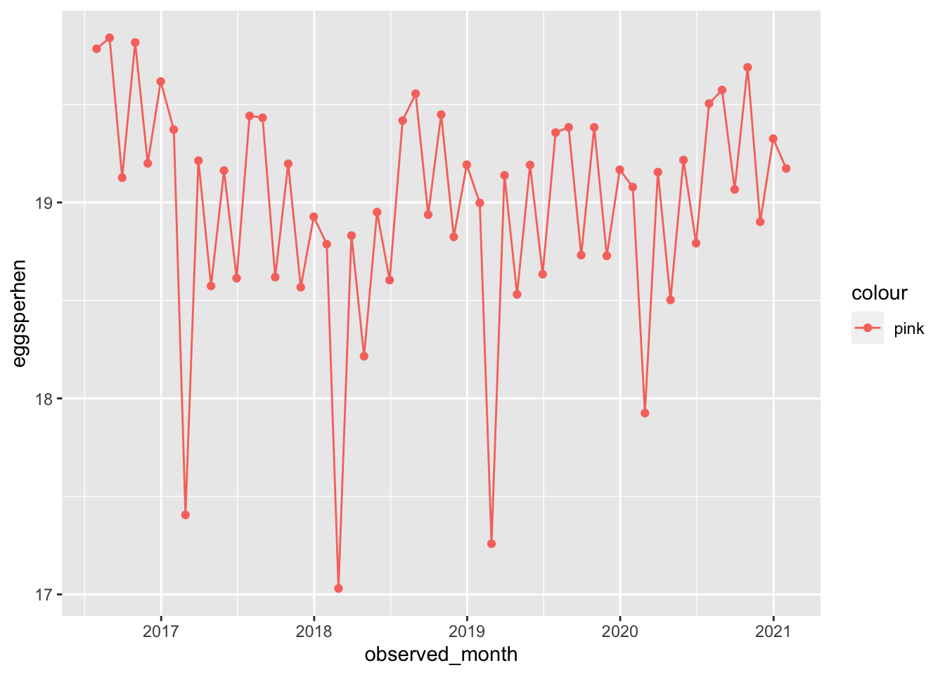
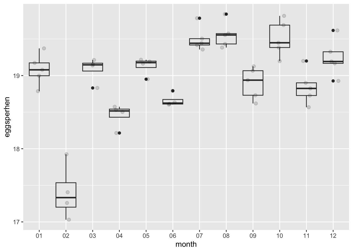
Looks like something is weird in February: the median # of eggs per month is closer to 17, compared to >18 in all other months. Maybe this is due to an increased desire for more table eggs in those months.
Maybe we’ll use this in our model. But lets also explore some table egg information.
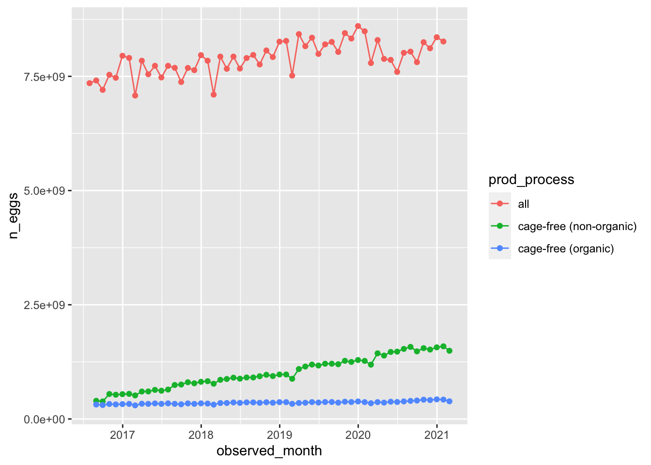
Lets look at the number of table eggs per hen over time
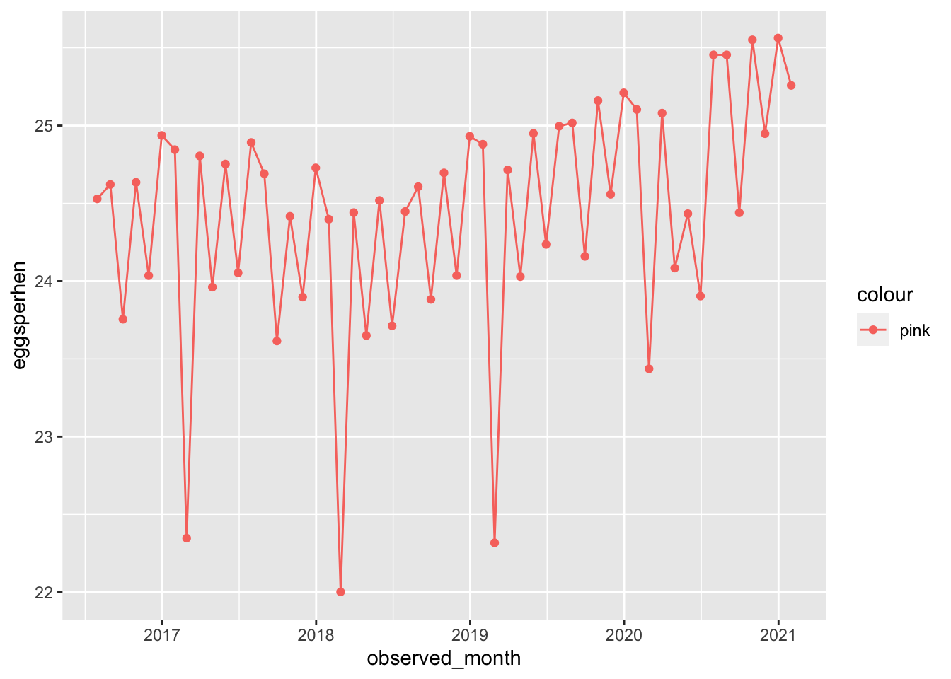
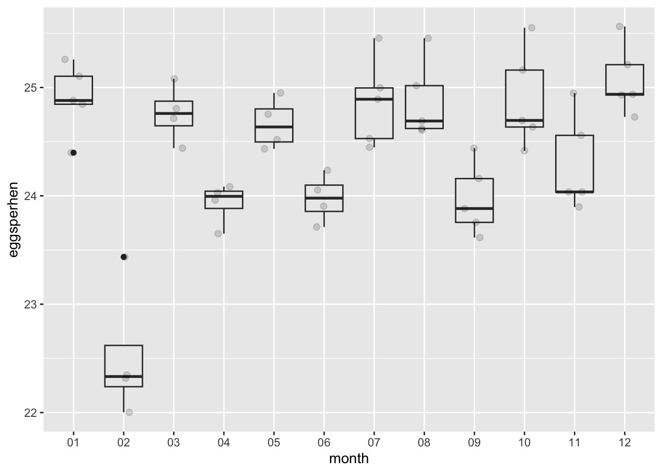
THe number of eggs per hen for table eggs is also lower in February! Strange. Its also interesting to note that the number of eggs per hen is much higher for table eggs than hatching eggs!
Lets also look at the number of table eggs in total over time
Interestingly, looks like all table eggs was on an upward trend… until 2020.
Cage free non-organic eggs seem to be increasing production faster than organic eggs
Some potential analyses:
Potential analysis: ITS model looking at linear trend in egg production until March 2020 (start of COVID-19 pandemic)
Difference in Difference model looking at slope of organic versus non-organic eggs
Lets look at a pre COVID-19 and post-COVID-19
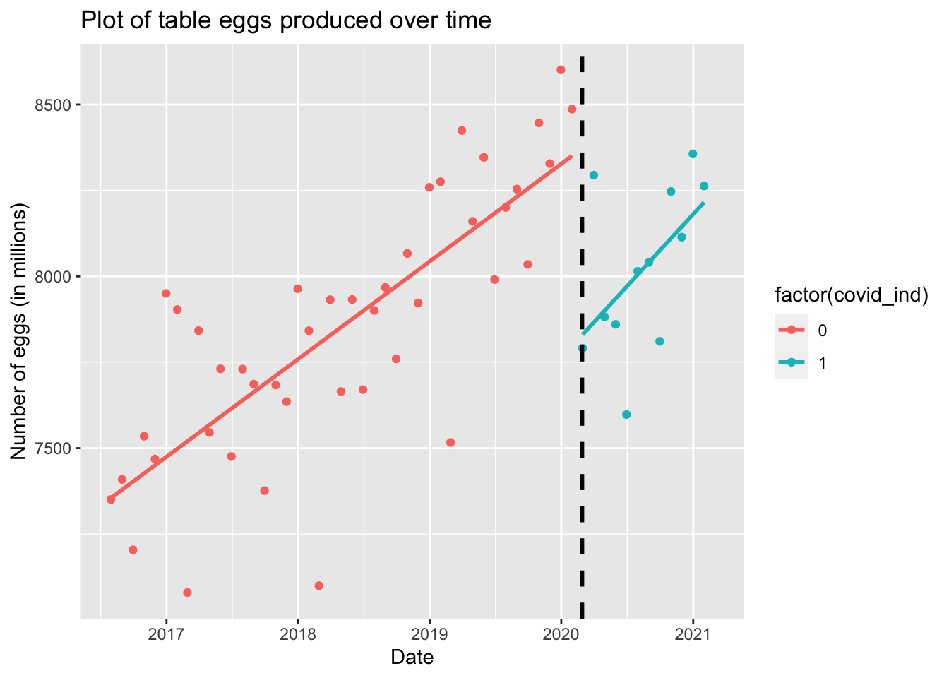
#Add covid indicator for any month in March 2020 forwardtableeggs2$cdate <-as.Date("2020-02-28")tableeggs2$covid_ind =ifelse(tableeggs2$observed_month>tableeggs2$cdate,1,0)tableeggs2$n_eggs_all_m <- tableeggs2$n_eggs_all/1000000tableeggs2$mindate =min(tableeggs2$observed_month)tableeggs2$daysmodel =as.numeric (tableeggs2$observed_month-tableeggs2$mindate)tableeggs2$interaction <-ifelse(tableeggs2$observed_month > tableeggs2$cdate,tableeggs2$daysmodel,0)#Plotting interrupted time series modelggplot(tableeggs2, aes(x=observed_month, y=n_eggs_all_m, group=factor(covid_ind),color=factor(covid_ind))) +geom_point() +geom_vline(xintercept = tableeggs2$cdate, linetype="dashed", color ="gray2", linewidth=1)+geom_smooth(method="lm", se=FALSE) +ggtitle("Plot of table eggs produced over time") +xlab("Date") +ylab("Number of eggs (in millions)")
Question: Was there a change in egg production related to the COVID-19 pandemic?
We are going to take an interrupted time series approach to understand if the linear trend in egg production changes beginning in March 2020, at the start of COVID-19 pandemic.
Here are my steps:
Data cleaning for the model: See above.
Assign 70% of data to training and 30% to test (make assignments by COVID_ind status so we have the same amount of data pre-post intervention)
Calculate linear regression with the following covariates: observed_month(month in time series), covid_ind (a 0/1 indicator variable for if in teh COVID-19 time period), and an interaction between covid_ind and observed_mont
Interpretation will be as follows:
Parameter (observed_month): Slope (Trend) before the pandemic
Parameter estimate (COVID_IND): Immediate change in egg production at start of pandemic
Parameter estimate (interaction term): Change in slope (trend) during the pandemic
Repeat model on test data to see if interpretation of parameter estimates are similar
── Conflicts ───────────────────────────────────────── tidymodels_conflicts() ──
✖ scales::discard() masks purrr::discard()
✖ dplyr::filter()   masks stats::filter()
✖ recipes::fixed()  masks stringr::fixed()
✖ dplyr::lag()      masks stats::lag()
✖ yardstick::spec() masks readr::spec()
✖ recipes::step()   masks stats::step()
• Dig deeper into tidy modeling with R at https://www.tmwr.org
library(performance)
Attaching package: 'performance'
The following objects are masked from 'package:yardstick':

    mae, rmse
set.seed(777)data_split <-initial_split(tableeggs2, prop =2/3, strata=covid_ind)# Create data frames for the two sets:train_data <-training(data_split)#36 obstest_data <-testing(data_split)#20 obsmodel_recipe <-recipe(n_eggs_all_m ~ daysmodel + covid_ind + interaction, data= train_data)#model: linear regression using GLM engineln_mod <-linear_reg() %>%set_engine ("lm")wflow <-workflow() %>%add_model(ln_mod) %>%add_recipe(model_recipe)#Fitting the model to train datasetmodel_fit_train <- wflow %>%fit(data = train_data)#Looking at model output;model_fit_train %>%extract_fit_parsnip() %>%tidy()
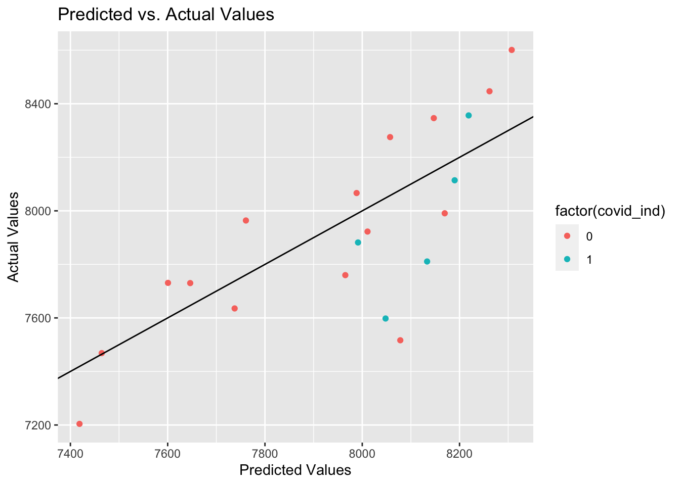
#augment dataaug <-augment(model_fit_train, test_data)#pull month and egg predictionobserved_daysmodel <- aug %>%pull(daysmodel)pred <- aug %>%pull(.pred)ggplot(aug, aes(x=.pred, y= n_eggs_all_m, group=factor(covid_ind), color=factor(covid_ind))) +geom_point() +geom_abline(intercept=0, slope=1) +labs(x='Predicted Values', y='Actual Values', title='Predicted vs. Actual Values')
#run rmsermse_vec(observed_daysmodel, pred)
[1] 7053.268
Summary of findings:
From our training dataset we estimate an increase of 0.74 million eggs per day prior to COVID-19. At the start of COVID-19 we saw an immediate decrease of 650 million eggs per day! Then, after COVID-19 we saw an increased trend of 0.18 million additional eggs per day (for a post-COVID-19 trend of 0.92 million more eggs produced each day!!).
Summary of our model fit:
In our plot of observed versus predicted values for the test data we feel confident that our model predicted well. There was potentially less good prediction in teh COVID-19 era than the pre-COVID-19 era but that is likely due to the small sample of data in that period for the model.