R Coding Exercise - Kelly Hatfield

R Code for loading packages

#load dslabs package
library("dslabs")
#load ggplot2
library(ggplot2)

#look at help file for gapminder data
help(gapminder)
#get an overview of data structure
str(gapminder)

'data.frame':   10545 obs. of  9 variables:
 $ country         : Factor w/ 185 levels "Albania","Algeria",..: 1 2 3 4 5 6 7 8 9 10 ...
 $ year            : int  1960 1960 1960 1960 1960 1960 1960 1960 1960 1960 ...
 $ infant_mortality: num  115.4 148.2 208 NA 59.9 ...
 $ life_expectancy : num  62.9 47.5 36 63 65.4 ...
 $ fertility       : num  6.19 7.65 7.32 4.43 3.11 4.55 4.82 3.45 2.7 5.57 ...
 $ population      : num  1636054 11124892 5270844 54681 20619075 ...
 $ gdp             : num  NA 1.38e+10 NA NA 1.08e+11 ...
 $ continent       : Factor w/ 5 levels "Africa","Americas",..: 4 1 1 2 2 3 2 5 4 3 ...
 $ region          : Factor w/ 22 levels "Australia and New Zealand",..: 19 11 10 2 15 21 2 1 22 21 ...

#get a summary of data
summary(gapminder)

                country           year      infant_mortality life_expectancy
 Albania            :   57   Min.   :1960   Min.   :  1.50   Min.   :13.20  
 Algeria            :   57   1st Qu.:1974   1st Qu.: 16.00   1st Qu.:57.50  
 Angola             :   57   Median :1988   Median : 41.50   Median :67.54  
 Antigua and Barbuda:   57   Mean   :1988   Mean   : 55.31   Mean   :64.81  
 Argentina          :   57   3rd Qu.:2002   3rd Qu.: 85.10   3rd Qu.:73.00  
 Armenia            :   57   Max.   :2016   Max.   :276.90   Max.   :83.90  
 (Other)            :10203                  NA's   :1453                    
   fertility       population             gdp               continent   
 Min.   :0.840   Min.   :3.124e+04   Min.   :4.040e+07   Africa  :2907  
 1st Qu.:2.200   1st Qu.:1.333e+06   1st Qu.:1.846e+09   Americas:2052  
 Median :3.750   Median :5.009e+06   Median :7.794e+09   Asia    :2679  
 Mean   :4.084   Mean   :2.701e+07   Mean   :1.480e+11   Europe  :2223  
 3rd Qu.:6.000   3rd Qu.:1.523e+07   3rd Qu.:5.540e+10   Oceania : 684  
 Max.   :9.220   Max.   :1.376e+09   Max.   :1.174e+13                  
 NA's   :187     NA's   :185         NA's   :2972                       
             region    
 Western Asia   :1026  
 Eastern Africa : 912  
 Western Africa : 912  
 Caribbean      : 741  
 South America  : 684  
 Southern Europe: 684  
 (Other)        :5586  

#determine the type of object gapminder is
class(gapminder)

[1] "data.frame"

R code for data exploration and cleaning

#Write code that assigns only the African countries to a new object/variable called africadata. 

africadata = subset(gapminder, continent=='Africa')

#Run str and summary on the new object you created.
str(africadata)

'data.frame':   2907 obs. of  9 variables:
 $ country         : Factor w/ 185 levels "Albania","Algeria",..: 2 3 18 22 26 27 29 31 32 33 ...
 $ year            : int  1960 1960 1960 1960 1960 1960 1960 1960 1960 1960 ...
 $ infant_mortality: num  148 208 187 116 161 ...
 $ life_expectancy : num  47.5 36 38.3 50.3 35.2 ...
 $ fertility       : num  7.65 7.32 6.28 6.62 6.29 6.95 5.65 6.89 5.84 6.25 ...
 $ population      : num  11124892 5270844 2431620 524029 4829291 ...
 $ gdp             : num  1.38e+10 NA 6.22e+08 1.24e+08 5.97e+08 ...
 $ continent       : Factor w/ 5 levels "Africa","Americas",..: 1 1 1 1 1 1 1 1 1 1 ...
 $ region          : Factor w/ 22 levels "Australia and New Zealand",..: 11 10 20 17 20 5 10 20 10 10 ...

summary(africadata)

         country          year      infant_mortality life_expectancy
 Algeria     :  57   Min.   :1960   Min.   : 11.40   Min.   :13.20  
 Angola      :  57   1st Qu.:1974   1st Qu.: 62.20   1st Qu.:48.23  
 Benin       :  57   Median :1988   Median : 93.40   Median :53.98  
 Botswana    :  57   Mean   :1988   Mean   : 95.12   Mean   :54.38  
 Burkina Faso:  57   3rd Qu.:2002   3rd Qu.:124.70   3rd Qu.:60.10  
 Burundi     :  57   Max.   :2016   Max.   :237.40   Max.   :77.60  
 (Other)     :2565                  NA's   :226                     
   fertility       population             gdp               continent   
 Min.   :1.500   Min.   :    41538   Min.   :4.659e+07   Africa  :2907  
 1st Qu.:5.160   1st Qu.:  1605232   1st Qu.:8.373e+08   Americas:   0  
 Median :6.160   Median :  5570982   Median :2.448e+09   Asia    :   0  
 Mean   :5.851   Mean   : 12235961   Mean   :9.346e+09   Europe  :   0  
 3rd Qu.:6.860   3rd Qu.: 13888152   3rd Qu.:6.552e+09   Oceania :   0  
 Max.   :8.450   Max.   :182201962   Max.   :1.935e+11                  
 NA's   :51      NA's   :51          NA's   :637                        
                       region   
 Eastern Africa           :912  
 Western Africa           :912  
 Middle Africa            :456  
 Northern Africa          :342  
 Southern Africa          :285  
 Australia and New Zealand:  0  
 (Other)                  :  0  

#We now have 2907 observations, down from 10545. Depending on how you do this, you might also notice that all the different categories are still kept in the continent (and other) variables, but show 0.

#Take the africadata object and create two new objects (name them whatever you want)

#Object 1 contains only infant_mortality and life_expectancy

myvars1 <- c("infant_mortality","life_expectancy")
object1 <- africadata[myvars1]
str(object1)

'data.frame':   2907 obs. of  2 variables:
 $ infant_mortality: num  148 208 187 116 161 ...
 $ life_expectancy : num  47.5 36 38.3 50.3 35.2 ...

summary(object1)

 infant_mortality life_expectancy
 Min.   : 11.40   Min.   :13.20  
 1st Qu.: 62.20   1st Qu.:48.23  
 Median : 93.40   Median :53.98  
 Mean   : 95.12   Mean   :54.38  
 3rd Qu.:124.70   3rd Qu.:60.10  
 Max.   :237.40   Max.   :77.60  
 NA's   :226                     

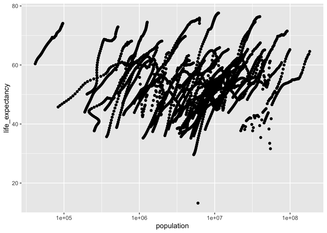
# Object2 contains only population and life_expectancy. 

myvars2 <- c("population","life_expectancy")
object2 <- africadata[myvars2]
str(object2)

'data.frame':   2907 obs. of  2 variables:
 $ population     : num  11124892 5270844 2431620 524029 4829291 ...
 $ life_expectancy: num  47.5 36 38.3 50.3 35.2 ...

summary(object2)

   population        life_expectancy
 Min.   :    41538   Min.   :13.20  
 1st Qu.:  1605232   1st Qu.:48.23  
 Median :  5570982   Median :53.98  
 Mean   : 12235961   Mean   :54.38  
 3rd Qu.: 13888152   3rd Qu.:60.10  
 Max.   :182201962   Max.   :77.60  
 NA's   :51                         

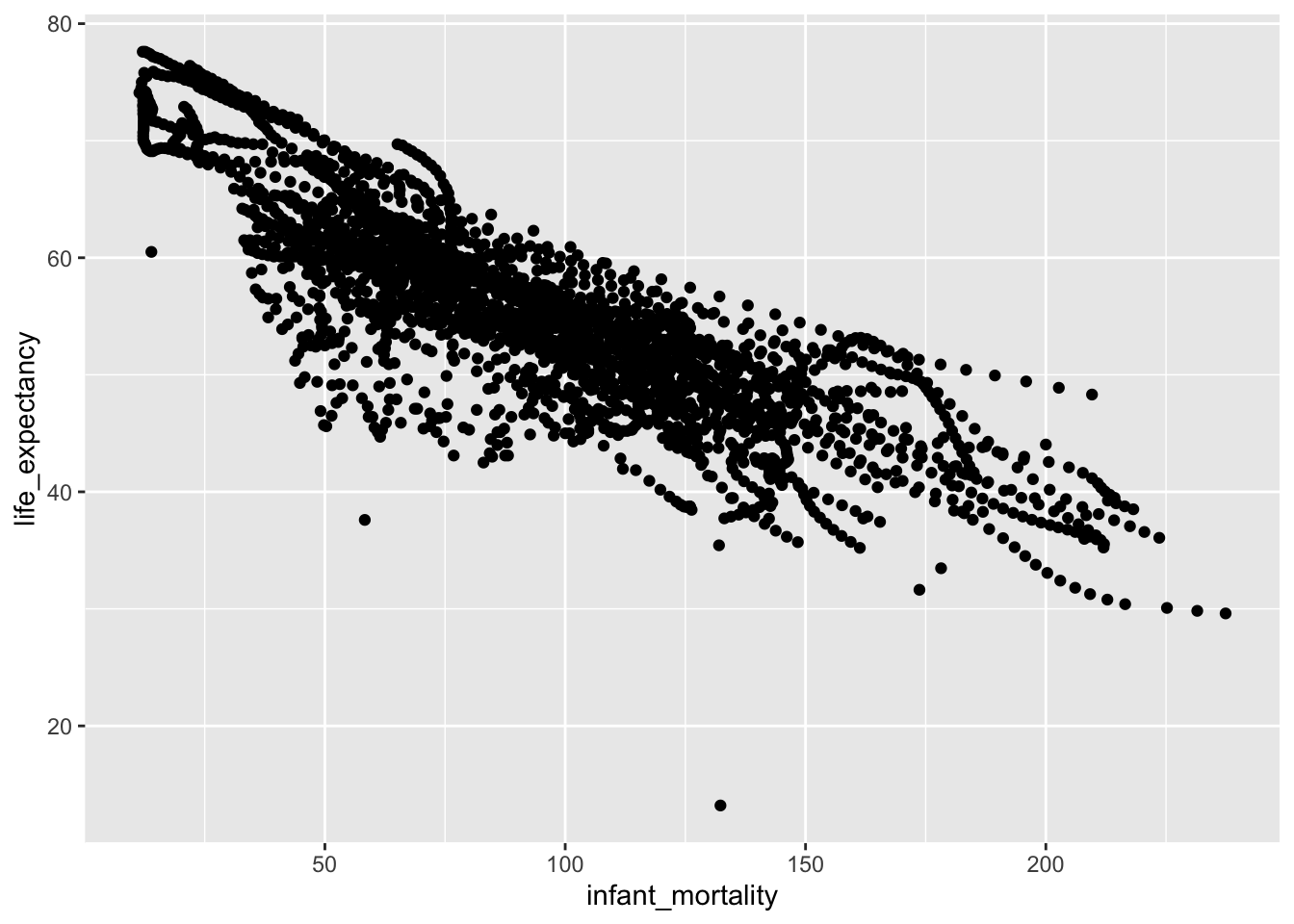
#Plot the data as points.
#Object 1
ggplot(object1, aes(x=infant_mortality, y=life_expectancy)) +geom_point()

Warning: Removed 226 rows containing missing values (`geom_point()`).

#Object2
p<- ggplot(object2, aes(x=population, y=life_expectancy)) +geom_point()
p + scale_x_continuous(trans = 'log10')

Warning: Removed 51 rows containing missing values (`geom_point()`).

#Looking at code for years with missing infant mortality
missing_mortality = subset(africadata, is.na(infant_mortality)) 
table(missing_mortality$year)

1960 1961 1962 1963 1964 1965 1966 1967 1968 1969 1970 1971 1972 1973 1974 1975 
  10   17   16   16   15   14   13   11   11    7    5    6    6    6    5    5 
1976 1977 1978 1979 1980 1981 2016 
   3    3    2    2    1    1   51 

Plotting and Analyzing Data from African Countries in 2000

#New Object just for Year=2000
africadata_2000 = subset(africadata, year==2000) 
str(africadata_2000)

'data.frame':   51 obs. of  9 variables:
 $ country         : Factor w/ 185 levels "Albania","Algeria",..: 2 3 18 22 26 27 29 31 32 33 ...
 $ year            : int  2000 2000 2000 2000 2000 2000 2000 2000 2000 2000 ...
 $ infant_mortality: num  33.9 128.3 89.3 52.4 96.2 ...
 $ life_expectancy : num  73.3 52.3 57.2 47.6 52.6 46.7 54.3 68.4 45.3 51.5 ...
 $ fertility       : num  2.51 6.84 5.98 3.41 6.59 7.06 5.62 3.7 5.45 7.35 ...
 $ population      : num  31183658 15058638 6949366 1736579 11607944 ...
 $ gdp             : num  5.48e+10 9.13e+09 2.25e+09 5.63e+09 2.61e+09 ...
 $ continent       : Factor w/ 5 levels "Africa","Americas",..: 1 1 1 1 1 1 1 1 1 1 ...
 $ region          : Factor w/ 22 levels "Australia and New Zealand",..: 11 10 20 17 20 5 10 20 10 10 ...

summary(africadata_2000)

         country        year      infant_mortality life_expectancy
 Algeria     : 1   Min.   :2000   Min.   : 12.30   Min.   :37.60  
 Angola      : 1   1st Qu.:2000   1st Qu.: 60.80   1st Qu.:51.75  
 Benin       : 1   Median :2000   Median : 80.30   Median :54.30  
 Botswana    : 1   Mean   :2000   Mean   : 78.93   Mean   :56.36  
 Burkina Faso: 1   3rd Qu.:2000   3rd Qu.:103.30   3rd Qu.:60.00  
 Burundi     : 1   Max.   :2000   Max.   :143.30   Max.   :75.00  
 (Other)     :45                                                  
   fertility       population             gdp               continent 
 Min.   :1.990   Min.   :    81154   Min.   :2.019e+08   Africa  :51  
 1st Qu.:4.150   1st Qu.:  2304687   1st Qu.:1.274e+09   Americas: 0  
 Median :5.550   Median :  8799165   Median :3.238e+09   Asia    : 0  
 Mean   :5.156   Mean   : 15659800   Mean   :1.155e+10   Europe  : 0  
 3rd Qu.:5.960   3rd Qu.: 17391242   3rd Qu.:8.654e+09   Oceania : 0  
 Max.   :7.730   Max.   :122876723   Max.   :1.329e+11                
                                                                      
                       region  
 Eastern Africa           :16  
 Western Africa           :16  
 Middle Africa            : 8  
 Northern Africa          : 6  
 Southern Africa          : 5  
 Australia and New Zealand: 0  
 (Other)                  : 0  

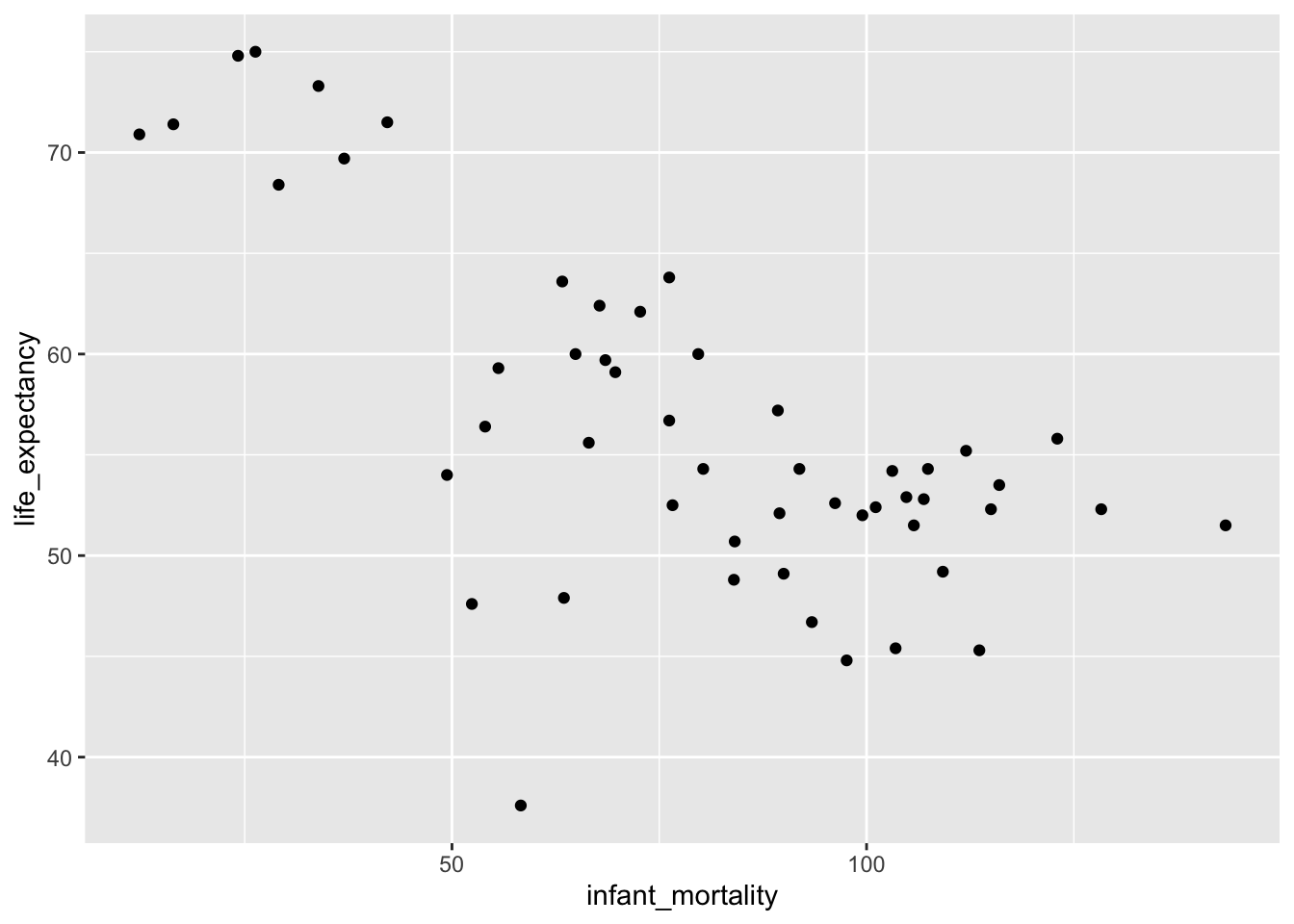
#More Plotting
#Infant Mortality and Life Expectancy in 2000;
ggplot(africadata_2000, aes(x=infant_mortality, y=life_expectancy)) +geom_point()

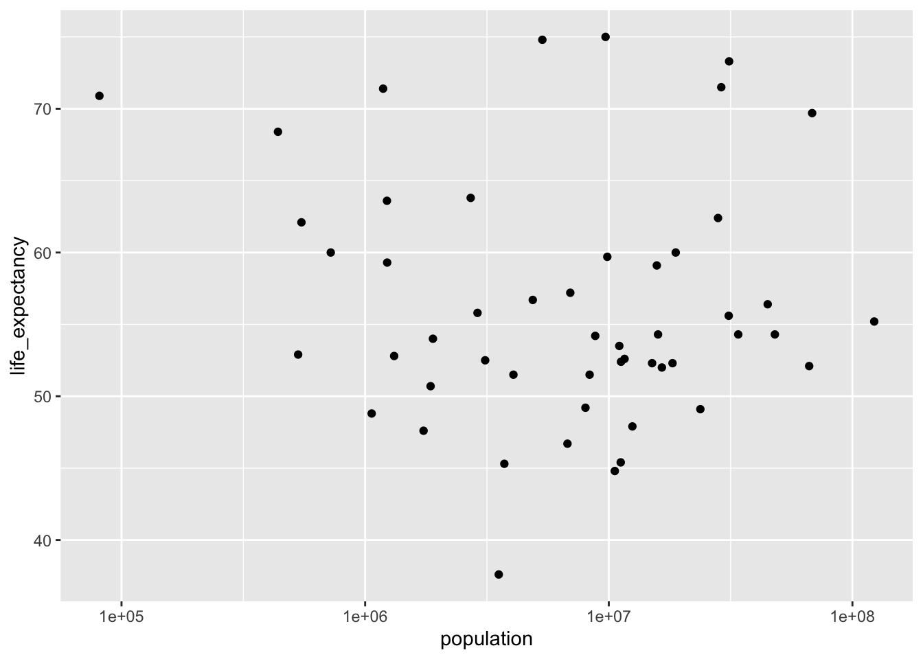
#Population and Life Expectancy in 2000; 
p2<- ggplot(africadata_2000, aes(x=population, y=life_expectancy)) +geom_point()
p2 + scale_x_continuous(trans = 'log10')

#Statistics
#fit linear regression model using 'x' as predictor and 'y' as response variable
fit1 = lm(life_expectancy~infant_mortality, data=africadata_2000)
summary(fit1)

Call:
lm(formula = life_expectancy ~ infant_mortality, data = africadata_2000)

Residuals:
     Min       1Q   Median       3Q      Max 
-22.6651  -3.7087   0.9914   4.0408   8.6817 

Coefficients:
                 Estimate Std. Error t value Pr(>|t|)    
(Intercept)      71.29331    2.42611  29.386  < 2e-16 ***
infant_mortality -0.18916    0.02869  -6.594 2.83e-08 ***
---
Signif. codes:  0 '***' 0.001 '**' 0.01 '*' 0.05 '.' 0.1 ' ' 1

Residual standard error: 6.221 on 49 degrees of freedom
Multiple R-squared:  0.4701,    Adjusted R-squared:  0.4593 
F-statistic: 43.48 on 1 and 49 DF,  p-value: 2.826e-08

fit2 = lm(life_expectancy~population, data=africadata_2000)
summary(fit2)

Call:
lm(formula = life_expectancy ~ population, data = africadata_2000)

Residuals:
    Min      1Q  Median      3Q     Max 
-18.429  -4.602  -2.568   3.800  18.802 

Coefficients:
             Estimate Std. Error t value Pr(>|t|)    
(Intercept) 5.593e+01  1.468e+00  38.097   <2e-16 ***
population  2.756e-08  5.459e-08   0.505    0.616    
---
Signif. codes:  0 '***' 0.001 '**' 0.01 '*' 0.05 '.' 0.1 ' ' 1

Residual standard error: 8.524 on 49 degrees of freedom
Multiple R-squared:  0.005176,  Adjusted R-squared:  -0.01513 
F-statistic: 0.2549 on 1 and 49 DF,  p-value: 0.6159

Conclusions

We determined that in a simple linear regression that increased life expectancy is associated with linear trend in decreased infant mortality for African countries in the year 2000. However, population size does not appear to have a linear relationship with life expectancy.

AK Edits

This section is added by Abbie Klinker to expand on Kelly’s findings.

I am interested at looking at infant mortality as it relates to fertility and population. The fertility measure is the number of children per woman. Infant mortality is recorded as the number of children <1yr old dead per 1000 live births.

I would predict that infant mortality is inversely related to fertility and population, while fertility and population are positively related to one another. This would mean that countries with higher rates of infant mortality have lower number of babies per woman and therefore a lower population. If this is proved untrue, then that would raise questions about access to resources like healthcare and quality of life.

Preparing the Data

First I’m going to see if all the data for these variables is still available for year 2000.

library(tidyverse)

── Attaching packages ─────────────────────────────────────── tidyverse 1.3.2 ──
✔ tibble  3.1.8      ✔ dplyr   1.0.10
✔ tidyr   1.3.0      ✔ stringr 1.5.0 
✔ readr   2.1.3      ✔ forcats 0.5.2 
✔ purrr   1.0.1      
── Conflicts ────────────────────────────────────────── tidyverse_conflicts() ──
✖ dplyr::filter() masks stats::filter()
✖ dplyr::lag()    masks stats::lag()

africadata%>%
  filter(year ==2000, 
         is.na(fertility)) #no data is missing for fertility in 2000, so we can still use this data.

[1] country          year             infant_mortality life_expectancy 
[5] fertility        population       gdp              continent       
[9] region          
<0 rows> (or 0-length row.names)

head(africadata_2000)#Kelly's created Africa 2000 data

          country year infant_mortality life_expectancy fertility population
7402      Algeria 2000             33.9            73.3      2.51   31183658
7403       Angola 2000            128.3            52.3      6.84   15058638
7418        Benin 2000             89.3            57.2      5.98    6949366
7422     Botswana 2000             52.4            47.6      3.41    1736579
7426 Burkina Faso 2000             96.2            52.6      6.59   11607944
7427      Burundi 2000             93.4            46.7      7.06    6767073
             gdp continent          region
7402 54790058957    Africa Northern Africa
7403  9129180361    Africa   Middle Africa
7418  2254838685    Africa  Western Africa
7422  5632391130    Africa Southern Africa
7426  2610945549    Africa  Western Africa
7427   835334807    Africa  Eastern Africa

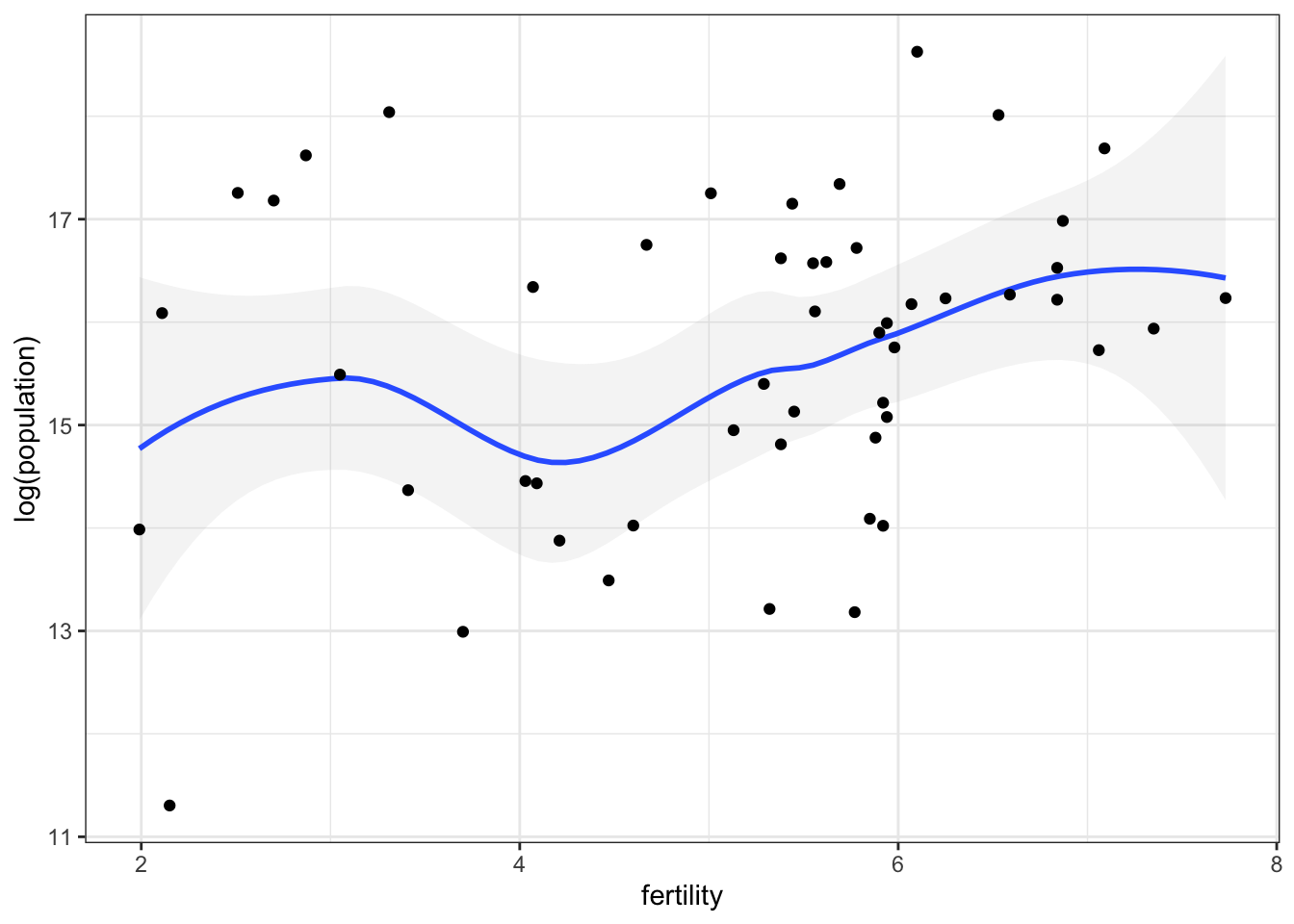
Since they are, I want to first look at how fertility may affect population.

Fertility vs. Population

ggplot()+
  geom_smooth(aes(y=log(population), x=fertility), data=africadata_2000, alpha = 0.1)+
  geom_point(aes(y=log(population), x=fertility), data=africadata_2000)+
  theme_bw()

`geom_smooth()` using method = 'loess' and formula = 'y ~ x'

There doesn’t seem to be much of a correlation for fertility versus population, at least using logs. I’ll double-check this quantitatively as well.

Regression Fertility vs Population

fit3 = lm(population~fertility, data=africadata_2000)
summary(fit3)

Call:
lm(formula = population ~ fertility, data = africadata_2000)

Residuals:
      Min        1Q    Median        3Q       Max 
-15760443 -12563579  -7667052   1295355 106245914 

Coefficients:
            Estimate Std. Error t value Pr(>|t|)
(Intercept) 10355760   11577157   0.894    0.375
fertility    1028697    2162449   0.476    0.636

Residual standard error: 22260000 on 49 degrees of freedom
Multiple R-squared:  0.004597,  Adjusted R-squared:  -0.01572 
F-statistic: 0.2263 on 1 and 49 DF,  p-value: 0.6364

Based on this regression model, as supported by the plot above, we don’t have evidence to support the associated between fertility alone and population. This is a bit surprising to me, because I would think that as the number of children per woman increased, so would the population.

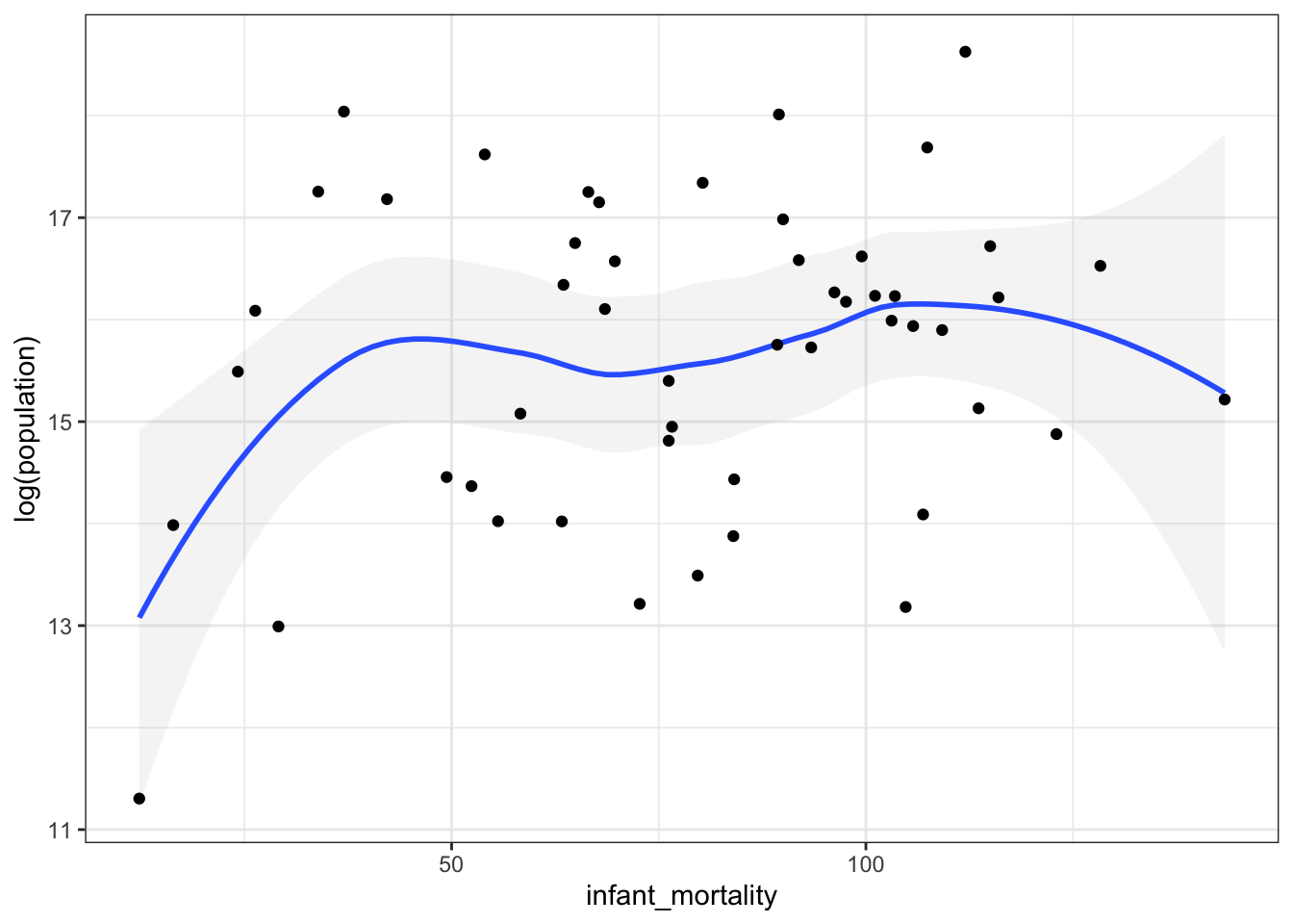
Now I want to look at infant mortality as a determinant of population.

Infant Mortality vs Population.

ggplot()+
  geom_smooth(aes(y=log(population), x=infant_mortality), data=africadata_2000, alpha = 0.1)+
  geom_point(aes(y=log(population), x=infant_mortality), data=africadata_2000)+
  theme_bw()

`geom_smooth()` using method = 'loess' and formula = 'y ~ x'

There also doesn’t seem to be much of a correlation for infant mortality versus population.

Regression Infant Mortality vs Population

fit4 = lm(population~infant_mortality, data=africadata_2000)
summary(fit4)

Call:
lm(formula = population ~ infant_mortality, data = africadata_2000)

Residuals:
      Min        1Q    Median        3Q       Max 
-16307667 -12769228  -7828854    733380 105710100 

Coefficients:
                 Estimate Std. Error t value Pr(>|t|)
(Intercept)      12063474    8682734   1.389    0.171
infant_mortality    45564     102671   0.444    0.659

Residual standard error: 22260000 on 49 degrees of freedom
Multiple R-squared:  0.004003,  Adjusted R-squared:  -0.01632 
F-statistic: 0.1969 on 1 and 49 DF,  p-value: 0.6592

And this is supported with the regression model as well. This is also surprising as I would guess that a country with higher rates of infant mortality would have a more stagnant population, while countries with lower rates would have a growing population.

Combined Variable Interactions

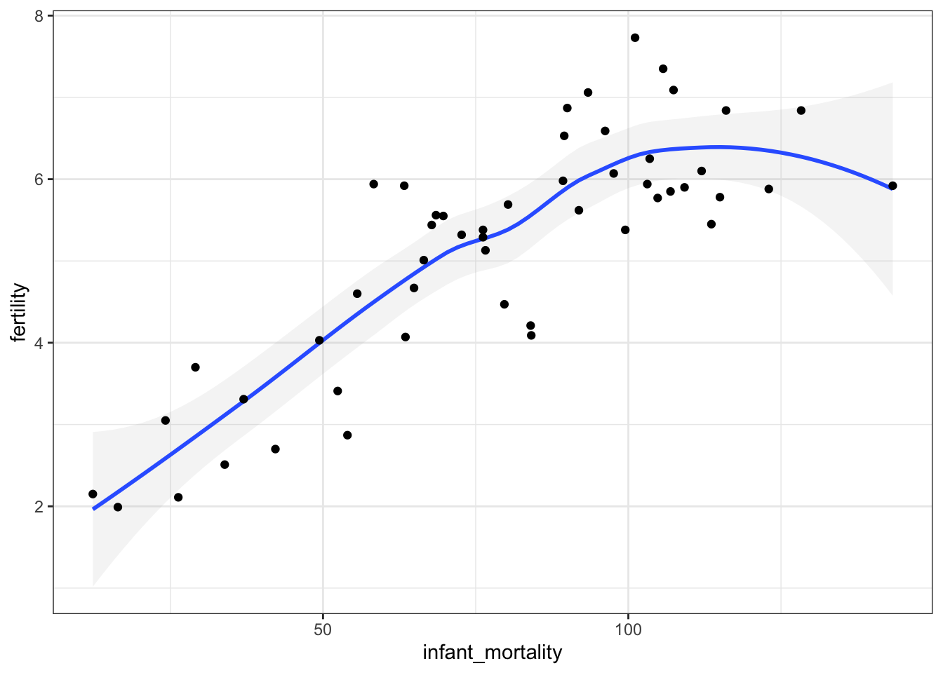
However, I want to see if infant mortality and fertility have an interaction, which together may impact the population.

Infant Mortality vs Fertility

ggplot()+
  geom_smooth(aes(x=infant_mortality, y=fertility), data=africadata_2000, alpha = 0.1)+
  geom_point(aes(x=infant_mortality, y=fertility), data=africadata_2000)+
  theme_bw()

`geom_smooth()` using method = 'loess' and formula = 'y ~ x'

It seems like there is a relationship here where they have a positive correlation, rather than the negative one which I had previously assumed. As the Gapminder documentation describes, this may be an indication of “many children and short lives.”

fit5<-lm(fertility~infant_mortality, data=africadata_2000)
summary(fit5)

Call:
lm(formula = fertility ~ infant_mortality, data = africadata_2000)

Residuals:
     Min       1Q   Median       3Q      Max 
-1.76037 -0.64424  0.04014  0.48908  1.70450 

Coefficients:
                 Estimate Std. Error t value Pr(>|t|)    
(Intercept)       2.06086    0.32306   6.379 6.08e-08 ***
infant_mortality  0.03921    0.00382  10.265 8.38e-14 ***
---
Signif. codes:  0 '***' 0.001 '**' 0.01 '*' 0.05 '.' 0.1 ' ' 1

Residual standard error: 0.8284 on 49 degrees of freedom
Multiple R-squared:  0.6826,    Adjusted R-squared:  0.6761 
F-statistic: 105.4 on 1 and 49 DF,  p-value: 8.379e-14

Combined Effect on Population

fit6<-lm(population~infant_mortality*fertility, data=africadata_2000)
summary(fit6)

Call:
lm(formula = population ~ infant_mortality * fertility, data = africadata_2000)

Residuals:
      Min        1Q    Median        3Q       Max 
-16611567 -11852919  -8981133   1442415 105324669 

Coefficients:
                           Estimate Std. Error t value Pr(>|t|)
(Intercept)                21941250   24539351   0.894    0.376
infant_mortality            -194248     437131  -0.444    0.659
fertility                  -1845199    6236486  -0.296    0.769
infant_mortality:fertility    41894      78706   0.532    0.597

Residual standard error: 22660000 on 47 degrees of freedom
Multiple R-squared:  0.01073,   Adjusted R-squared:  -0.05242 
F-statistic: 0.1699 on 3 and 47 DF,  p-value: 0.9162

The combined effect still does not have an association with population, nor is the interaction between the two variables significant. Since they are correlated, this may be a case of multicolinearity, which I will double check just to be sure:

library(car)

Loading required package: carData

Attaching package: 'car'

The following object is masked from 'package:dplyr':

    recode

The following object is masked from 'package:purrr':

    some

vif(fit6)

there are higher-order terms (interactions) in this model
consider setting type = 'predictor'; see ?vif

          infant_mortality                  fertility 
                 17.505466                   8.027358 
infant_mortality:fertility 
                 34.057197 

The standard cutoff for VIF use is 10, so since the interaction between infant mortality and fertility is a whopping 34, we can assume this is a redundant term and should not be used in a model.

Remove the Interaction

fit62<-lm(population~infant_mortality+fertility, data=africadata_2000)
summary(fit62)

Call:
lm(formula = population ~ infant_mortality + fertility, data = africadata_2000)

Residuals:
      Min        1Q    Median        3Q       Max 
-16010329 -12607659  -7840265    950724 105972070 

Coefficients:
                 Estimate Std. Error t value Pr(>|t|)
(Intercept)      10533816   11864479   0.888    0.379
infant_mortality    16457     184056   0.089    0.929
fertility          742243    3877752   0.191    0.849

Residual standard error: 22490000 on 48 degrees of freedom
Multiple R-squared:  0.004763,  Adjusted R-squared:  -0.03671 
F-statistic: 0.1149 on 2 and 48 DF,  p-value: 0.8917

vif(fit62)

infant_mortality        fertility 
        3.150547         3.150547 

Now that we’ve removed the interaction, while the model still does not show any significant associations between population, infant mortality, and fertility, we can be confident in our answers and the validity of the model.

Conclusions

Based on this analysis, we can conclude that neither infant mortality or the number of children per woman influence a country’s population. However, countries with higher rates of infant mortality also have more children per woman. Based on this data, for every child dead per 1000 live births, the average woman is likely to have 0.04 more children. This is not a very interpretable number. When translated, this can also mean that when the infant mortality rate reaches 1 in 40 live births (0.025%), the average woman will have 1 child. While this may seem insanely high, based on the data, 16 countries have infant mortality rates over 100, or 1 death per in 10 births, and in these countries the average number of children per woman is over 6, and we see this average drop to around 4 in the countries with lower infant mortality rates. This is an indication of lack of access to resources like reproductive healthcare, education, and necessities like food and water.

Thanks

Thanks to Abbie Klinker for her awesome additional analyses!